Reading Your Generated Portfolio

This page explains how to read the results screen of the CleaRank Portfolio Generator. Each run gives you six frontier variants, a walk-forward test on data the optimizer never saw, a Monte Carlo simulation of the years ahead, and a replay through real market crises. Below is every number on that screen, what a good value looks like, and what to change when it is bad.

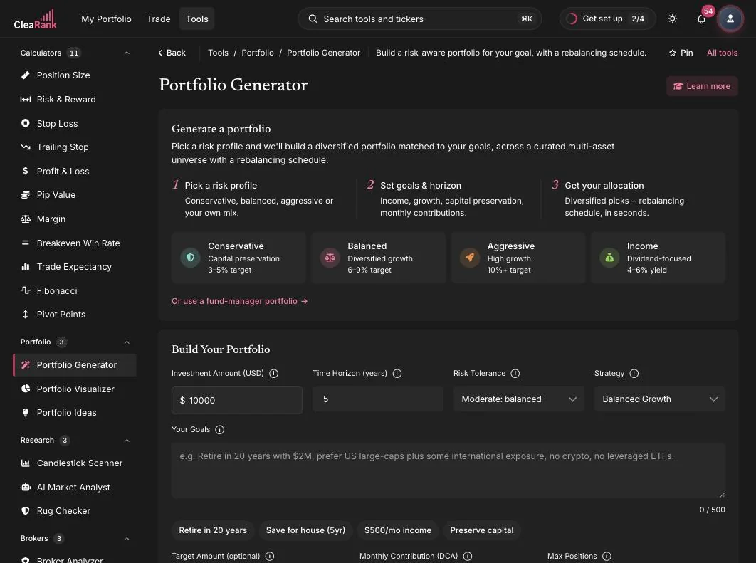
The inputs that change the answer

Most people set the amount and the horizon and stop. The six fields below change the shape of the result far more than the dollar amount does.

The four quick profiles

The first-run card offers four profiles, and each one fills in risk tolerance and strategy for you. The Conservative profile targets capital preservation with a 3 to 5 percent annual goal. Balanced targets diversified growth at 6 to 9 percent. Aggressive targets high growth at 10 percent and above. The Income profile is the one people miss: it is dividend focused and targets a 4 to 6 percent yield, which is a different objective from total return. Pick Income when you need the portfolio to pay you while you hold it, and expect a lower headline growth number in exchange. Every field stays editable after you pick a profile.

Target Amount and Monthly Contribution

Target Amount is optional. Set it and the Generator runs an extra simulation to estimate the probability of reaching that figure inside your horizon, plus a feasibility check that says whether the target is realistic at all. There is no official pass mark on that probability. Read anything under 50 percent as the plan telling you the target is not funded by this mix. Only three levers move it: raise the monthly contribution, extend the horizon, or lower the target. Raising risk usually widens the range of outcomes without moving the median much.

Monthly Contribution (DCA) defaults to zero, and leaving it there is the most common way to make a plan look worse than it is. Contributions are added month by month inside every simulated path, not bolted on at the end. The tool’s own worked example: 500 dollars a month for 20 years adds about 120,000 dollars of capital before any growth at all.

Max Positions, leveraged ETFs and factor tilts

Max Positions caps how many tickers survive into the final allocation. It accepts 6 to 30 and defaults to 20, and 10 to 20 is the usual working range. Fewer positions means each one carries more of the outcome. More positions means more rebalancing friction for diminishing diversification benefit, because the tenth broad-market ETF adds very little the first three did not. The optimizer also holds each surviving position roughly between 2.5 percent and 30 percent of the portfolio, so a very small Max Positions will produce chunky weights by construction.

Allow leveraged ETFs is off by default. Turning it on adds UPRO, TQQQ, SSO and TMF to the candidate pool and caps total leveraged exposure at 25 percent of the portfolio.

Include factor tilts is on by default. It adds momentum (MTUM), value (VLUE), quality (QUAL), low volatility (USMV) and size (SIZE) to the candidate pool. Switch it off if you want a plainer broad-market and bond mix with no style bets in it.

The six frontier variants

Every run produces six allocations from the same candidate pool, each solving a different problem. They are not ranked. The point is that you can see what the trade-offs cost.

• Defensive (lowest volatility). The minimum-variance allocation: the mix whose combined swing is the smallest that the assets allow. It is not required to beat the benchmark, so it often trails it. Pick it when the size of the drawdown matters more to you than the size of the return.
• Balanced (best risk-adjusted return). The maximum-Sharpe allocation, pulled toward a market-equilibrium starting point so that one asset with a lucky run cannot take over the weights. It is constrained to at least match the benchmark.
• Aggressive (highest return). Targets a return above the Balanced mix and is constrained to clear the benchmark by a margin. The on-screen tagline reads “Highest return, +5% over benchmark”. Read that as the ambition, not a promise: what the optimizer enforces is a minimum margin over the benchmark on historical data, and future returns are whatever the assets deliver.
• Alpha-Hunter (maximum alpha versus benchmark). Optimizes on active returns, meaning each asset measured as its excess over the benchmark rather than its raw return. That is the information-ratio objective. Use it when your question is specifically “what beats the index”, not “what has the best standalone numbers”.
• Risk Parity (equal risk per asset). Sizes each position so it contributes the same amount of risk, rather than the same amount of money. A small bond sleeve and a large equity sleeve are not equal risks, and this variant corrects for that. It is not required to beat the benchmark.
• Hierarchical (cluster-robust diversification). Groups the assets by how they actually move together, then allocates down that tree. It avoids the instability that pure matrix methods hit when two holdings are near-identical. You will sometimes see this approach abbreviated HRP elsewhere. It is not required to beat the benchmark.

All six are long-only, and all six are produced by resampling: the optimizer solves the same problem many times on bootstrapped stretches of history and averages the answers, so one unusual period cannot set your weights by itself. Do not choose between them on headline return. Choose on the out-of-sample block below.

The walk-forward out-of-sample test

This is the most important block on the page and the easiest to skip. The optimizer is shown only the earlier part of the history and chooses weights from it. Those weights are then scored on the later part, which it never saw. Any allocation can look excellent on the data used to build it. Only the out-of-sample numbers tell you whether it was fitted to signal or to noise.

Three figures are reported.

• Out-of-sample Sharpe. Return per unit of volatility, measured above a 4.5 percent risk-free rate. Under 1 is weak, 1 to 2 is solid, 2 to 3 is strong, and above 3 on a multi-year sample almost always means a short window or leverage rather than skill. The comparison that matters is in-sample versus out-of-sample: a Sharpe of 2.1 that falls to 0.4 out of sample is an overfitted portfolio, not a good one.
• Out-of-sample return. Judge it against the benchmark’s return over the same test window, never against an absolute target. A 6 percent result is excellent in a year the benchmark did 2 percent and poor in a year it did 18 percent.
• Beat-Benchmark Frequency. The share of overlapping rolling windows in which the portfolio’s compounded return beat the benchmark’s. The headline results use one-year windows of 252 trading days, stepped one day at a time. The out-of-sample block uses a shorter window, roughly three to six months, because the test slice is shorter. 50 percent is a coin flip. Below 50 percent the benchmark was the better holding more often than not, and the extra complexity is not earning its keep. Above 50 percent, look at how far above and across how many windows, because 60 percent over 40 windows and 60 percent over 4 windows are not the same finding.

When out-of-sample results collapse, the usual fixes are to lower Max Positions, turn leverage off, lengthen the period, and favor Defensive, Risk Parity or Hierarchical. Those three do not need an estimate of future returns to work, which is exactly the estimate that overfits.

Bootstrap confidence intervals

Where a metric is shown as a range rather than a single figure, that range comes from a block bootstrap. History is resampled in 21-day blocks, so roughly a month of market behavior stays intact instead of being shuffled day by day, the metric is measured again on each resample, and the spread of those answers becomes the interval. The optimizer runs the same procedure across 40 to 60 resamples when it averages the weights.

The width is the whole point. A Sharpe of 1.4 with an interval of 1.2 to 1.6 is a finding. A Sharpe of 1.4 with an interval of 0.1 to 2.7 is a coin toss with a decimal point on it. If an interval straddles zero, this sample has not established the metric at all, and the fix is a longer period or a simpler portfolio rather than a different variant.

Diversification Ratio and average pairwise correlation

The Diversification Ratio is the weighted sum of the individual holdings’ volatilities divided by the volatility of the portfolio as a whole. It cannot go below 1.00. Exactly 1.00 means your holdings gave you nothing: you own one bet in several wrappers, and the mix swings as hard as its parts. Anything meaningfully above 1.00 means the holdings’ moves partly cancel, and the further above it sits, the more of the individual risk the combination is absorbing.

Average pairwise correlation is the average correlation across every pair of holdings, on a scale from -1 (they move exactly opposite) through 0 (unrelated) to +1 (identical). As a working rule, an average above about 0.8 means your holdings are close substitutes, and the Diversification Ratio will stay near 1.00 no matter how many more tickers you add. The fix is a structurally different exposure, such as bonds, commodities or non-US equity, rather than another ticker from the same sector.

The Monte Carlo projection

The projection is a distribution of possible futures, not a forecast. These are the settings behind it.

• Fat-tailed by design. Returns are drawn from a Student-t distribution with 5 degrees of freedom rather than a normal bell curve, so extreme days show up at something closer to the rate real markets produce them. The scale is corrected so the historical variance is preserved.
• 1,500 paths are simulated on every run.
• The horizon is your Time Horizon in years multiplied by 252 trading days.
• Monthly contributions are inside the simulation, added along every path rather than added to the result.
• The drift is blended: 60 percent from the portfolio’s own historical daily mean and 40 percent from a valuation-adjusted forward estimate. A decade of unusually strong returns therefore cannot be projected forward unchallenged.
• Correlations come from history. The simulation runs on the already-weighted portfolio return series, so the relationships between holdings are baked in from the real data rather than redrawn each path.
• The Target Amount probability comes from the same run as the projection bands, so the two figures can never disagree with each other.

Read the median as the middle outcome, not the expected one, and spend most of your attention on the lower band. If the pessimistic path leaves you short of what the money is for, the plan is not robust however good the median looks.

Valuation-adjusted forward returns and the Market Regime card

The forward half of that drift blend is adjusted using CAPE, a valuation measure that divides price by average inflation-adjusted earnings over ten years so a single boom or bust year does not distort it. High CAPE readings have historically preceded weaker long-run returns and low readings stronger ones. This is why the projection is usually more conservative than a straight extrapolation of the backtest, and why a portfolio that returned 18 percent a year for five years will not be projected forward at 18 percent.

The Market Regime card puts that projection in current context using a broad equity index, an equity volatility index, long-dated government bonds and a market sentiment reading. It describes the environment the projection starts from. It is context for your judgment, not a timing signal, and it does not change your allocation.

The stress eras

Your allocation is replayed through six named periods:

• Dot-com Crash, March 2000 to October 2002
• Global Financial Crisis, October 2007 to March 2009
• COVID Crash, February to March 2020
• COVID Recovery, March to August 2020
• Tech Drawdown, January to October 2022
• Rate-Cut Rally, October 2023 to July 2024

An era only runs if the price history available for your tickers covers it. Because that history is sized to your chosen period, the Dot-com Crash and the Global Financial Crisis are skipped on almost every run. That is honest reporting rather than a fault, and skipped eras are listed explicitly so you never mistake a missing test for a passed one.

In each era that does run, look at the drawdown before the return. If your allocation lost more through the COVID Crash than you could sit through, you will not hold it through the next one, and an allocation you abandon halfway is worse than a duller one you keep.

Which benchmark you are actually being measured against

The default benchmark is the S&P 500 (SPY), but it follows your Strategy: Conservative Income is measured against a broad bond index (AGG), Dividend Growth against SCHD, Balanced Growth against a diversified allocation fund (AOR), Global Diversified against ACWI, Aggressive Growth against SPY, and Tech and Innovation against QQQ. A Conservative Income portfolio that “beats the benchmark” beat a bond index, not the stock market. Check the benchmark named on your results before you draw any conclusion about beating the market.

The risk metrics

• VaR (95%) is a one-day figure: the loss level that only the worst 5 percent of days in the period exceeded. A reading of 1.8 percent means about one trading day in 20 was worse than -1.8 percent. It is not scaled up to weeks or years. Use it to check whether the day-to-day noise is something you can live with.
• CVaR (95%) is the average loss across those worst 5 percent of days, so it is always at least as large as VaR. It answers the question that matters in a crisis: when it is bad, how bad. A wide gap between VaR and CVaR means the left tail is long, and the occasional day is much worse than the threshold suggests.
• Beta is how much the portfolio moved for each 1 percent move in the benchmark. 1.00 moves with it, 0.50 moves half as much, above 1.00 amplifies it. It is shown as unavailable when fewer than 30 overlapping days of data exist, because there is not enough to estimate it honestly.
• Alpha is the annualized return above what the portfolio’s beta alone would have earned, after allowing for a 4.5 percent risk-free rate. Positive alpha means the mix contributed something beyond plain market exposure. A small positive alpha on a short sample is noise, so read it next to its confidence interval, not on its own.
• Sortino is a risk-adjusted return that counts only downside deviation. Read it on the same scale as Sharpe: under 1 weak, 1 to 2 solid, 2 to 3 strong. It is normally higher than Sharpe because upside volatility is not penalized, and a large gap between the two tells you most of the movement was upward. It is shown as unavailable when the portfolio had effectively no downside in the period, which is a signal that the sample is too calm to judge, not a perfect score.
• Max drawdown is the deepest peak-to-trough fall inside the period, measured on the compounded curve. This is the number investors actually abandon plans at: a 20 percent or deeper drawdown is where most people capitulate. If yours is larger than anything you have personally sat through, size down or move toward Defensive or Risk Parity.

What the numbers do and do not include

• Every return figure is a total return including reinvested dividends. Fund expense ratios are already reflected in the prices used, so the weighted expense ratio shown beside the allocation is informational and is not subtracted a second time.
• If a headline annual figure looks pinned at 25 percent, that is a deliberate cap on forward-looking guidance rather than the historical result. The uncapped historical figure is what other CleaRank portfolio views show.
• A ticker needs at least 60 daily closes to be optimized. Ones with fewer than 30 are reported back to you as missing data rather than quietly dropped. If fewer than four tickers survive, the run stops and asks you to regenerate.
• The Generator builds from a curated, strategy-specific pool of broad-market, sector, factor and bond ETFs plus a set of mega-cap single names. It is not a whole-market screen. To test a specific ticker list of your own, use the Portfolio Visualizer, which accepts any ticker it can find price history for.

For a plain-language summary of the tool without signing in, see the Portfolio Generator page on clearank.com.

Frequently asked questions

Related articles

CleaRank tools are for education and analysis. Nothing in this guide is financial advice.